Pipelining graph execution
Introduction
There’re two things I need to describe before describing actual solution.
Why graphs and optimization criteria are like this
Because that’s a solution that I wanted to suggest at work (for a well-described problem), but the solution will probably be rejected. So the problem is not very abstract.
Why don’t I refer to other solutions
The problem at hand is very specific, and, despite it being (as I believe) very common for some systems (say, optimizations for compilers), finding any solutions will take a lot of time (and a lot of reading). I have just one week, and I’m not an expert on optimizing program execution.
Also, as my solution won’t actually be used anywhere, why not to try to invent a wheel just to do a mental exercise?
The problem
Can be described as “execution graph pipelining and optimization”, but that’s just the tip of the iceberg.
What graphs are
Graphs to be discussed are what I call “execution graphs”.
These graphs follow these rules:
- Graphs are not planar.
- Edges are directional
- There’s only one output (final result) node, but there’re many input nodes.
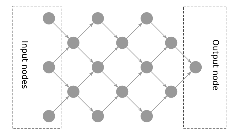
- Every possible path can only contain one reference to each node in that path. i.e. there’re no cyclic dependencies. Thus CFG-based solutions are not relevant – there’re no “control” nodes.
- Every node (except input nodes and output node) can have multiple inputs and multiple outputs. That makes it a bit different from common AST, because those have only one output per node.
- (This one is obvious, but) no node can start execution before all of it’s dependencies (node inputs) are resolved.
- Every node returns all values at once, so, once node finished executing – all it’s outputs are available.
- There’re “external nodes” (E-nodes), that could not be executed within the system. For example, filesystem reads or external execution systems.
Some specifics
- Nodes operate on “reasonably” large chunks of data: ~100mb each, which makes passing them through like plain values (say, uint32 numbers) not an option and these chunks should be stored in (pre)allocated buffers.
- All chunks of data are of the same size (or could be easily padded to be)
- Each node internal memory and computation consumption is not considered.
- It’s rare that some graph contains more than 50 nodes, with potential cap at 100 nodes. For now.
What I’m trying to achieve
There’re multiple goals, described in order of importance
- Grouped E-node execution, so that context switching (between internal and external execution) is minimized.
- Static execution. No dynamic allocations, no dynamic execution. Strong execution plan and exact amount of memory preallocated.
- Memory optimization. Do not allocate memory for every node result, but only those required for next node(s) execution.
- Potentially parallelization. If some (sub)paths have the same input or external dependencies, but no interconnections, execute these subpaths concurrently.
- Potentially E-node result caching if these are considered expensive.
There’s one thing to have in mind: compilation time and memory consumption is not pretty critical, because such compilation will be performed way less often than graph execution.
The solution
Grouping E-nodes and internal nodes (I-nodes)
The simplest solution to the problem of static execution is graph linearization, because there’re too many algorythms designed for 1-dimensional structures (lists). But, without further analysis it could not be executed concurrently.
Primitive linearization could be achieved by simply ordering nodes by dependencies like this:
If node A depends on node B, node A should be placed after node B (A depends on B -> A > B).
If node B depends on node A, node B should be placed after node A (B depends on A -> B > A).
If neither node A nor node B depend on one another they are considered equal order-wise (A ⊥ B -> A == B).
By definition they could not depend on each other, so the rule above will ensure any node is executed after it’s dependencies.
That condition could be further expanded to group E-nodes:
If node A depends on node B, node A should be placed after node B (A depends on B -> A > B).
If node B depends on node A, node B should be placed after node A (B depends on A -> B > A).
If node A is an internal node and B is an E-node, node A should be placed after node B (A: E-node, B: I-node -> A > B).
If node B is an internal node and A is an E-node, node B should be placed after node A (B: E-node, A: I-node -> B > A).
If neither node A nor node B depend on one another and have the same type they are considered equal order-wise (A ⊥ B -> A == B).
Since input nodes are not fully “executed” (they only contain input values), they could be excluded from that ordering and put in any order at the beginning of the list.
Since E-nodes are grouped, it makes sense to build plans for each internal-node block.
So, top-level plan will contain alternating blocks of internal nodes (I-blocks) and E-nodes (E-blocks).
Naive planning and memory management
Obviously, memory management only should be done for I-blocks.
At the beginning of every internal-node block data should be “imported” into memory from either some initial data or I-block results (which are stored), then, at the end of I-block, it should be exported from memory to storage (making it possible to either output final result or execute E-nodes).
For naive case we assume, that every operation is non-destructive – does not change data in input buffers.
Then, simplest method of getting some preallocated memory and strong plan would be to use dynamic “dry run” with these rules:
- Buffers will be managed by using “dynamic” pool to which we can add, but not remove. Initially it’s empty.
- Buffers containing data should be marked with node and output name the data came from. Empty buffers will be marked as “empty”.
- Every input node will put data into a new buffer (thus, +1 buffer per input node).
- The system will need to provide a buffer per each requested output for every node when executing that node (getting requested outputs is pretty simple – won’t describe it here). If there’re free buffers – these buffers should be used, otherwise a new buffer should be added to the pool.
- Every time buffer is not used as an input in non-finished I-block node it’s considered “free” and should be emptied – either by just marking it as free, or by explicitly running nullifying procedure on that buffer. Such check should be executed after each node execution.
- When all nodes are finished – nonempty buffers should be “exported” to storage as I-block result.
When building the final plan, all allocations should be moved to the beginning.
So, a simple set of commands could be used:
Allocate buffer (id: $buffer_id)(orAllocate buffersif that is possible)Import (from: $node_id, output_name: $output_name, to: $buffer_id)Run node (inputs: {$input_name: $buffer_id, ...}, outputs: {$output_name: $buffer_id, ...})Free buffer (buffer: $buffer_id), which will do nothing if all node implementations fully rewrite buffer contentExport (from: $buffer_id, node_id: $node_id, output_name: $output_name)
Where all $ marked values will be inlined by the compiler when performing dry run.
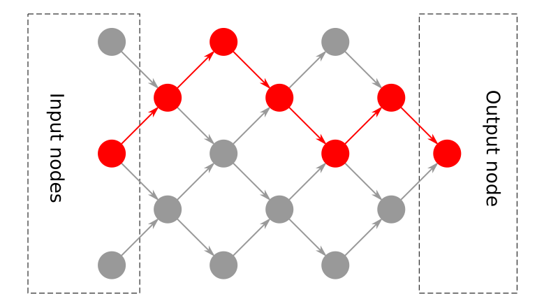
Resulting plan for that graph will look like this:
Allocate buffers | {"count": 5}
Import node data | {"node": "1", "output_name": "data", "to": 0}
Import node data | {"node": "2", "output_name": "data", "to": 1}
Import node data | {"node": "3", "output_name": "data", "to": 2}
Run node         | {"node": "4", "input": {"data": 0}, "output": {"another data": 3, "data": 4}}
Free buffer      | {"id": 0}
Run node         | {"node": "5", "input": {"data 1": 1, "data 2": 2}, "output": {"data": 0}}
Free buffer      | {"id": 1}
Free buffer      | {"id": 2}
Run node         | {"node": "6", "input": {"data": 4}, "output": {"data": 1}}
Free buffer      | {"id": 4}
Run node         | {"node": "7", "input": {"data": 3}, "output": {"data": 2}}
Free buffer      | {"id": 3}
Run node         | {"node": "8", "input": {"data": 0}, "output": {"data": 3}}
Free buffer      | {"id": 0}
Run node         | {"node": "9", "input": {"data": 1}, "output": {"data": 0}}
Free buffer      | {"id": 1}
Run node         | {"node": "10", "input": {"data 1": 2, "data 2": 3}, "output": {"data": 1}}
Free buffer      | {"id": 2}
Free buffer      | {"id": 3}
Run node         | {"node": "11", "input": {"data 1": 0, "data 2": 1}, "output": {"data": 2}}
Export node data | {"from": 2, "node": "11", "output_name": "data"}
As you can see, it’s a bit unoptimal: there’s no need to free buffers at the end of execution, potentially too many buffers allocated, but that’s why it’s called “naive”: it does the thing the simplest way possible.
Real planning and memory management
Now, that’s really complicated.
Each node can have multiple inputs and multiple outputs. Not only that, node behaviour per-input and per-output might be different depending on the implementation:
- Destructively put output to one of input buffers thus losing all the original data stored in input buffer. Generating such output does not require additional “output” buffer.
- Non-destructively put output to a new buffer. While original values are not overritten and could be used in another node, this will require additional buffer for that output.
- Both situations depending on requested outputs for a single node.
The exact behaviour should then be described in node spec.
That makes things messed up, because if, for example, there’re two nodes using some output destructively, the system should make a copy of an output to another buffer. If, on the other hand, no nodes use some output destructively, after all non-destructive nodes using the output are done, that output buffer should be reused.
For now I do not have enough time to come up with appropriate solution, please use the “naive” one that does not support destructive nodes.
TBD
- Do something on parallelization
- Support finite non-conditional (enumerated) loops.